
An issue here is that sensitivity in our case dictates a logical AND condition. That is, the waveform must be below AND above the respective sensitivity lines before it triggers. A trigger with a large hysteresis window may then fail to see even extreme highs and/or lows unless they both occur in a single acquisition.
Hi Ben,
thanks a lot for Your update 3.61
regarding the measurement-values,
there is a new idea (now the last one)
Top Bar displays the trigger, so we have
Bottom Bar with 3 Measurement Values selectable:
left: with left bottom
middle value: with OK
right: with right bottom
BenF
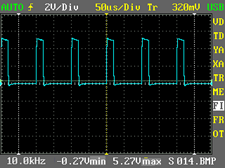
While preparing a video lesson for v3.61 I noticed an ambiguity, maybe you can help. FR = 1Khz, and is fed into the input channel of the Nano. In the attached zip file, Image001.bmp shows the fast sample time results and Image002.bmp shows the results for normal sample time. I can understand the Measured Freq being in error, but I don’t understand why the waveform amplitude changes. If you change the FR freq from 1Khz down to 300hz in steps, then the waveform amplitude increases in steps and reaches proper amplitude at 300hz. The Measurement Vmin and Vmax remain accurate for both fast and normal samples, only the displayed amplitude changes. The gif files shown below are the same as the bmp files in the zip.
The saved XML buffer file shows proper waveform amplitude, so the problem may be related to the screen display updates. File001.xml is also in the zip file.
The problem also exists at 10ms/Div. I understand that you wouldn’t normally look at this waveform in this manner but maybe you can identify what is going on and that could be helpful in other situations.
fast.zip (19 KB)
This is a result of compression (time domain) and averaging (voltage domain). The waveform area is 300 pixels wide and 200 pixels high. Each vertical column (one of 300) represents the average of all samples collected between the equivalent start and end time for this column. Time interval represented by a single display column is TDiv / 25 and when in fast sampling mode we collect some 10 samples during this short interval.
If we stop the waveform and increase T/Div further, the display will approach a straight horizontal line at Vavg and ultimately we end up with a single pixel at Vavg that represents the full sampling buffer (all 4098 samples).
There are many alternative schemes we could use to render a time domain compressed waveform including down sampling (normal vs. fast will illustrate this), min/max, peak and a whole range of more exotic approaches. Averaging is reasonably fast to compute (remember there is no $100 graphics processor in our Nano’s) and provides for a clean, noise reduced waveform display. All schemes however have their perks and typically a high end scope will allow us to choose between several alternatives.
One thing to keep in mind is that the actual samples (the raw data we collect during acquisition) are what is used for measurement calculations and so remain unaffected by any scheme we use for display rendering purposes.
Given the images posted by lygra I think an appropriate reaction would be to realize that the choice of T/Div is inappropriate for the displayed waveform and so adjust the controls (reduce T/Div) until we can clearly distinguish individual waveform cycles on the display.
Thanks for that thorough explanation. I figured it was in the display process and I have also seen the flat line condition you described. Now I know what is causing it.
Although the example compression of T/Div may be inappropriate while looking at a square wave, it could be appropriate while looking at the modulation of an AM modulated signal. Now I understand that while looking at an AM modulated waveform, you could enter this region of inaccurate displayed waveform amplitude and the amplitude should be confirmed. A quick range adjustment of T/Div steps to confirm that the amplitude remains constant, would be appropriate.
Hi
Discovered one little thing I could not do with the nano even with Bens greatest 3.61 (gosh is it really possible  I wanted to look at a echo from a ultrasonic flow meter. There are two transducers that constantly send a pings to each other. The ping is about a volt but the response from the other transducer is only a few millivolts and I could not get the oscilloscope to trigger on only the response. A nice feature would have been some kind of explicit trigging I guess that would trigger only if the top of the curve is within the trigging range, not over and not under but the signal has to start falling again inside this range.
Don’t know if it is a standard oscilloscope feature called something else or if it might be useful for any other scenarios also. Might be me just getting an idea I surely can live without such a feature, just wanted to hear if there was someone else who think it might be useful.
Anyway it turned out that there is not enough bandwidth to look at the signal I wanted to look at anyway as it is just one sample on the screen on lowest t/div.
No way, - if you follow the manual it will cook your dinner and do the dishes afterwards.
Isolating the received pulse from the transmitted pulse is a challenge as the frequency is likely to be the same and also the amplitude of the first and last couple of cycles from the transmitted pulse may very well match the received pulse amplitude. Neither frequency nor amplitude can then uniquely distinguish the transmitted signal from the received signal.
A reliable trigger mechanism may have to consider multiple cycles and then we’re well on the way to create a flow meter. Still I expect there will be all kinds of issues with echo from particles flowing in the liquid, pipe walls and so forth making this quite a challenge (I guess this is why the good ones cost an arm and a leg). I know some of these devices are based on detecting Doppler shifts, but this would probably require high resolution timing beyond the capability of our Nano’s.
One general approach to similar measurement challenges is to trigger on the transmitted pulse and then offset trigger position so that you observe the echo (or the pulse from the secondary transducer) rather than the initial pulse.
What is the distance between the transducers? The results will be based upon one ping and echo although an averaged value would be more accurate for the reasons stated by BenF.
If the distance traveled is sufficient, then connect both the transmitter and receiver to a single Nano channel, use a resistor summing network with attenuation towards the transmitter and no attenuation towards the receiver. Now you can slide the transmitter trigger to the left using Trig Pos and use the T2 cursor to measure the received pulse time offset position shown in the bottom right hand display position of the Nano.
Or NOT 
Hi
Distance is 1.067m. No distance is not the interesting thing, its the shape and amplitude of the ping. The frequency was to high anyway so I only see one or two samples a little higher on the nano at smallest t/div and v/div, no nicely shaped sinus curve 
Anyway the problem fixed itself, probably there was some minor blockage in the pipe in front of either of the transducers. It’s a common problem we have with other ultrasonic flow meters but it was the first time on this one where the flowrate is so high that blockage should be almost impossible.
Btw, we have dopplers also, extremly expensive and does not work when you got a sediment layer covering them so they require a clean canal and constant cleaning. They also have a built in pressure transmitter so it can calculate the flow if it knows the canal dimensions.
Hi!
Not having Scan at 50ms is becoming really annoying for me. I came to a point, where it is impossible to see spikes or other happenings in the signal. At 50ms and fast mode there is a part that is drawn “beside the screen” which i cannot see, but when i change to 100ms or 200ms the spike or even sine signals can´t be seen.
I really cant get along with this.
I would really appreciate if the Scan mode could be activated for all T/Div´s.
The feature I would most like to see on the nano is a waveform invert option - so I can invert ignition waveforms on ignition systems. I think this would be very useful. Other than that I think Benf has done a really good job with the firmware, and I dont think he could make a whole lot of more improvements with it, The rest of the ‘problems’ people are running into are hardware and not firmware limitations it seems to me. At first when I installed the firmware I had a couple of hangups, but after I renstalled it I havent had any problems. Very good job Benf.
How hard would it be to make a “invert waveform” function?
Why not take a step back and show us your waveform (such as an XML capture and screen dump) and point out what you try to detect.
When running the Nano on internal battery power, switching probes (plus/minus) will have this effect.
BenF’s suggestion to reverse the test leads is a very good solution when that is possible. Some of the automotive HV AC probes have a BNC connector which makes this reversal technique impractical when used with a BNC to mini-phone jack adapter.
Although this reversal feature would be nifty, is it really required? Ignition waveforms are normally used for cylinder comparisons at a glance and this can be done with the signal upside-down. The time and voltage cursors are just as effective for signal measurements even when the signal is upside-down. Any defective noise that may be present upon the signal can be observed and or measured while the image is inverted.
On your side of the coin, it might just be an easy implementation that BenF would consider for applications where the lead reversal is not practical.
That’s my 2-cents worth.
Oh well, i give up and maybe sell it.
A partially blind oszilloscope isnt that good.
It would be more productive to just provide an XML file as BenF has asked for. There is enough support here to help you if we know what you are trying to do. The Nano with BenF’s firmware is quite powerful and can probably do what you want in another mode of operation. If you would like some assistance in providing this XML file, just send a private message to lygra.
Hi.
Maybe I missed something.
Is the actual source code available for changes, enhancementes etc? (FFT, Protocols, …)
Thanks for your great work, regards,
Eduardo
In version 3.61, the buffer indicator at the bottom of the screen. What does the yellow filled box represent? It goes away while scrolling the buffer and then returns once the scrolling has stopped. The yellow outline box most likely represents the viewing window of the display but the solid box inside puzzles me.
Thanks
The outline is as you suggest, the viewing window and the solid box represents how buffer data is distributed (size and position) within this window. The “blinking” you see when repositioning trigger is just an unintentional artifact relating to how the display is refreshed.
Some small input.
Trigger Kind is typically called Trigger Edge or simply as a submenu item Edge.
Trigger Sensitivity := Trigger Hysteresis or Hysteresis
Regards.
Hello. While writing code.google.com/p/benfwaves/ I am looking for more information on vertical resolution of the DSO Nano V2. Specifically:
-
How do I determine vertical resolution? Is it affected by volts/div, or the attenuation field?
-
In the “Buffer Usage and Priority” section, it says that in fast sample mode, sampling rate can be increased at the expense of reduced sampling depth. Does this affect vertical resolution?
-
It says that the purpose of the sampleDiv field is to distinguish between normal and fast mode. However, for time scales below 50 us, it seems that there is no difference between the fast mode sampling frequency and the normal mode sampling frequency. Will a difference still show up between sampleDiv and timeDiv in the XML? If not, how does one detect fast mode in that case?
Thanks.